Pandas Tutorial
Course of Network Softwarization
Machine Learning for Networking
University of Rome “Tor Vergata”
Lorenzo Bracciale
Data manipulation with pandas
This is a short tutorial on main Pandas functions. Please refer to the official website for a more in-depth guide on Pandas.
credits: most of the material has been taken by the following tutorials.
import pandas as pd
Creating dataframes
The most important data structure in Pandas is the DataFrame which essentially is a table.
Let us create our first dataframe
pd.DataFrame({'A': [1, 2], 'B': [3, 4]})
| A | B | |
|---|---|---|
| 0 | 1 | 3 |
| 1 | 2 | 4 |
In this example, we set the names of the columns as “A” and “B”.
The names of the rows, in this example “0” and “1”, have been assigned by default and are called “indexes”.
We can explicitly specify the index of the dataframe in this way:
pd.DataFrame({'A': [1, 2], 'B': [3, 4]}, index=['X', 'Y'])
| A | B | |
|---|---|---|
| X | 1 | 3 |
| Y | 2 | 4 |
There exists also another data structure called Series, which is essentially a list, or we can see it as a column of a table.
pd.Series([1, 2]) # with automatic indexes
0    1
1    2
dtype: int64
Like in the dataframe, we can specify the index of the Series as well. Moreover, we can also specify the name of the Series.
pd.Series([1, 2], index=['A', 'B'], name='Product A') # with manual indexes and a name
A    1
B    2
Name: Product A, dtype: int64
Each Series has a data type (dtype). In the example above it was int64, but we can decide to create a Series with categoritcal data such as the next one, which will be assigned to the dtype object.
pd.Series(["good", "good", "bad", "good"])
0    good
1    good
2     bad
3    good
dtype: object
We can access to values and indexes of Series and Dataset in this way:
df = pd.DataFrame({'A': [1, 2], 'B': [3, 4]})
print("Values of the dataframe")
print(df.values) # this returns a numpy array

print("\nIndex of the dataframe")
print(df.index)
Values of the dataframe
[[1 3]
 [2 4]]

Index of the dataframe
RangeIndex(start=0, stop=2, step=1)
Typically series and dataframes are big and you need to import them automatically from a file.
You can also load your dataset from many formats like CSV, json or Excel:
#pd.read_csv('/your/path/file.csv')
#pd.read_excel('/your/path/file.xlsx')
#pd.read_json('/your/path/file.json')
Indexing and selecting data
Let us start by creating a simple testing dataframe to play with, and assign it to the variable df
df = pd.DataFrame({'A': [1,2,3], 'B': [4,5,6]}, index=['X', 'Y', 'Z'])
To view only the first lines (5 by default) we can use the head method. Likewise, to see the last lines of the dataframe we could use the tail method.
df.head()
| A | B | |
|---|---|---|
| X | 1 | 4 |
| Y | 2 | 5 |
| Z | 3 | 6 |
When we do machine learning, it is very important to understand the dimension of the dataset which is readily provided by the shape attribute:
df.shape
(3, 2)
We can then access to a specific column as
df['A'] # <-- this returns a Series
X    1
Y    2
Z    3
Name: A, dtype: int64
or using the next method
df.A
X    1
Y    2
Z    3
Name: A, dtype: int64
We can get the value of a specific cell in this way:
df['A']['X'] # <-- this returns a value
1
For more advanced indexing, we can resort to the following attributes:
loc: selection by labeliloc: selection by position
We can select our data based on its numerical position with iloc:
print("** First row **")
print(df.iloc[0])

print("\n ** First row, First column **")
print(df.iloc[0,0])


print("\n** Second column **")
print(df.iloc[:,1])
** First row **
A    1
B    4
Name: X, dtype: int64

 ** First row, First column **
1

** Second column **
X    4
Y    5
Z    6
Name: B, dtype: int64
Or use label-based selection with loc:
df.loc['X', 'A']
1
We create expressions such as the following one. Please note that the result is a column of boolean values
df['A'] > 1
X    False
Y     True
Z     True
Name: A, dtype: bool
We can then use this column to select only a subset of our dataset.
For instance, with the next command we select only the rows where the value of the “A” column is greater than 1.
df[df['A'] > 1] # only the second raw displayed
| A | B | |
|---|---|---|
| Y | 2 | 5 |
| Z | 3 | 6 |
Another usefull selection function is isin to check if the values are inside a given list
df['A'].isin([1,5,9])
X     True
Y    False
Z    False
Name: A, dtype: bool
Finally we will add a new column to an existing dataset.
To add (or replace) a column with constant value you can simple make the new column equal to a single value
df['D'] = 0
df
| A | B | D | |
|---|---|---|---|
| X | 1 | 4 | 0 |
| Y | 2 | 5 | 0 |
| Z | 3 | 6 | 0 |
Conversely, if you want to provide all the values of the new column, you can write:
import numpy as np
df['C'] = np.arange(3) # equals to [0, 1, 2]
df['D'] = ['Good', 'Bad', 'Bad'] #categorical data
df
| A | B | D | C | |
|---|---|---|---|---|
| X | 1 | 4 | Good | 0 |
| Y | 2 | 5 | Bad | 1 |
| Z | 3 | 6 | Bad | 2 |
# Usefull methods
Pandas is full of usefull methods to understand what is going on with your data.
For instance, to show some statistics about the current dataset we can use describe
df.describe()
| A | B | C | |
|---|---|---|---|
| count | 3.0 | 3.0 | 3.0 |
| mean | 2.0 | 5.0 | 1.0 |
| std | 1.0 | 1.0 | 1.0 |
| min | 1.0 | 4.0 | 0.0 |
| 25% | 1.5 | 4.5 | 0.5 |
| 50% | 2.0 | 5.0 | 1.0 |
| 75% | 2.5 | 5.5 | 1.5 |
| max | 3.0 | 6.0 | 2.0 |
We can call different statistical methods on any given column such as mean, std, min or max. For instance:
df['A'].mean()
2.0
Unique returns the value set of a columns. For instance, the set of unique values of column “D” are “Good” or “Bad”:
df['D'].unique()
array(['Good', 'Bad'], dtype=object)
value_counts is also very used since it give us the occurences of all the values:
df['D'].value_counts() #Two bad elements, good just one element
Bad     2
Good    1
Name: D, dtype: int64
## Modify values
It is common to apply a certain function to all the values of a column.
This is easily done with the apply method. For instance we could want to make a square out of a column, like this:
df['C'].map(lambda p: p * p)
X    0
Y    1
Z    4
Name: C, dtype: int64
Please note that most of these functions do not modify the original dataset!
df['C'] # it is not changed!
X    0
Y    1
Z    2
Name: C, dtype: int64
To actually change the column we can assign the modified dataframe such as:
df['C'] = df['C'].map(lambda p: p * p)
We can also call apply on each row. We are going to experiment with only the numerical part of our dataset (first three columns) since it would raise an exception if we launch it on a categorical column such as column “D”.
df[['A', 'B', 'C']].apply(lambda p: p * p, axis='columns')
| A | B | C | |
|---|---|---|---|
| X | 1 | 16 | 0 |
| Y | 4 | 25 | 1 |
| Z | 9 | 36 | 4 |
## Grouping
We can group our rows and then performing some calculation (e.g., count or min) on the fields:
df.groupby('D').count()
| A | B | C | |
|---|---|---|---|
| D | |||
| Bad | 2 | 2 | 2 |
| Good | 1 | 1 | 1 |
Data types
All the columns of our dataframe is a Series, and each Series has a data type (dtype)
df['A'].dtype
dtype('int64')
df.dtypes # to watch all the dtypes
A     int64
B     int64
D    object
C     int64
dtype: object
We can change the datatype with astype. For instance:
df['A'].astype('float64')
X    1.0
Y    2.0
Z    3.0
Name: A, dtype: float64
When we import a csv in pandas, it automatically try to guess the right datatype. Most of the time it does a very good job, however sometimes it can be usefull to force the dtype on some column. Please refer to the official docs of pandas to know more.
## Not a Number
It is common to do not have all the data.
In such cases, pandas fills the missing values with Not a Number value, aka NaN.
We are going to simulate this case:
df["E"] = np.nan, np.nan, 1  #simulate a columns with two missing values
df
| A | B | D | C | E | |
|---|---|---|---|---|---|
| X | 1 | 4 | Good | 0 | NaN |
| Y | 2 | 5 | Bad | 1 | NaN |
| Z | 3 | 6 | Bad | 2 | 1.0 |
isnull and notnull are two usefull selectors for such null values
print(pd.isnull(df['E']))
print("*********")
print(pd.notnull(df['E']))
X     True
Y     True
Z    False
Name: E, dtype: bool
*********
X    False
Y    False
Z     True
Name: E, dtype: bool
How to do machine learning with NaN?
It is not uncommon we need to substitute a constant value in place of all the NaN.
This is readily done by the fillna method.
df.fillna(42)
| A | B | D | C | E | |
|---|---|---|---|---|---|
| X | 1 | 4 | Good | 0 | 42.0 |
| Y | 2 | 5 | Bad | 1 | 42.0 |
| Z | 3 | 6 | Bad | 2 | 1.0 |
Or we can decide to drop the lines with `NaN``
df.dropna()
| A | B | D | C | E | |
|---|---|---|---|---|---|
| Z | 3 | 6 | Bad | 2 | 1.0 |
Concat, join, merge, split
Concat concatenates pandas objects along a particular axis (rows or columns)
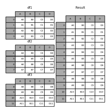
df1 = pd.DataFrame({'A': ['AO', 'A1'], 'B': ['B0', 'B1'], 'C': ['C0', 'C1']})
df2 = pd.DataFrame({'A': ['A2', 'A3'], 'B': ['B2', 'B3'], 'C': ['C2', 'C3']})

print("DataFrame1")
print(df1)

print("\nDataFrame2")
print(df2)

print("\nConcat of DF1 and DF2")
print(pd.concat([df1, df2]))
DataFrame1
    A   B   C
0  AO  B0  C0
1  A1  B1  C1

DataFrame2
    A   B   C
0  A2  B2  C2
1  A3  B3  C3

Concat of DF1 and DF2
    A   B   C
0  AO  B0  C0
1  A1  B1  C1
0  A2  B2  C2
1  A3  B3  C3
concat can be done on rows (by default, as in the example above), or on columns.
As happens for many Pandas commands, we can specify that with the axis parameter, where:
axis=0: means “do that for rows”axis=1: means “do that for columns”
print(pd.concat([df1, df2], axis=1)) #concat the columns
    A   B   C   A   B   C
0  AO  B0  C0  A2  B2  C2
1  A1  B1  C1  A3  B3  C3
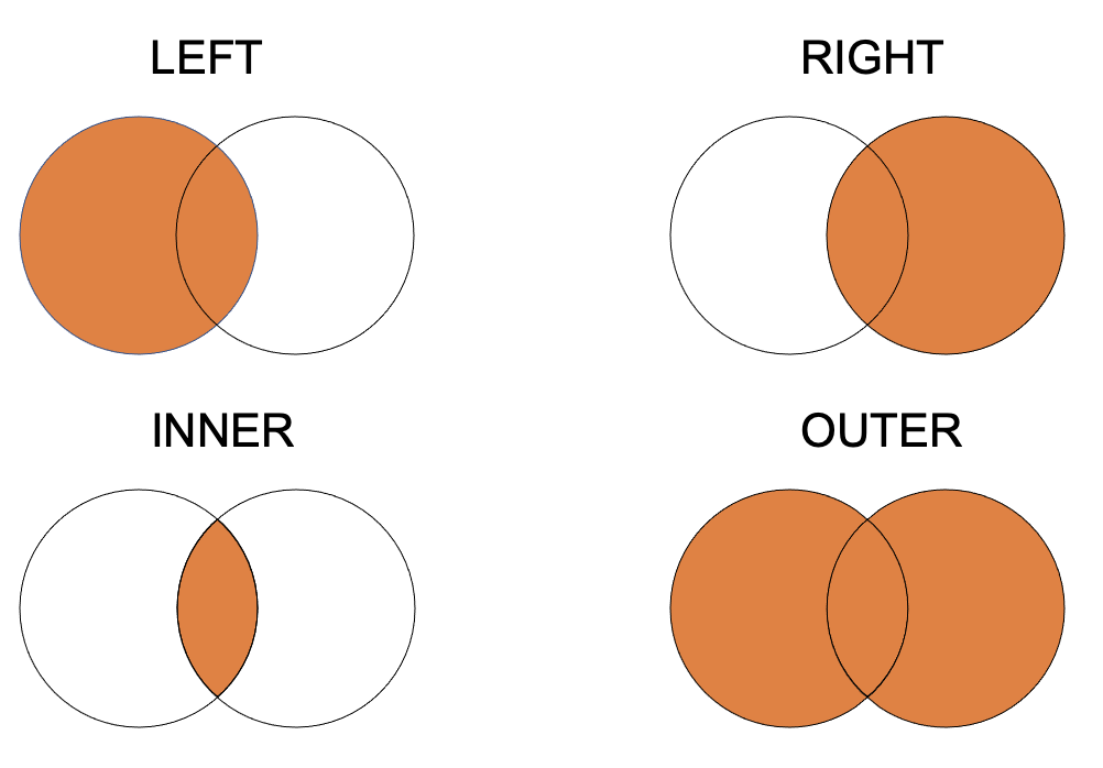
merge is more complicated since there are many forms of join:
- inner join: It returns a dataframe with only those rows that are on both dataframes. This is similar to the intersection of two sets.
- outer join: returns all those records which either have a match in the left or right dataframe.
- left join: returns a dataframe containing all the rows of the left dataframe. All the non-matching rows of the left dataframe contain NaN for the columns in the right dataframe.
- right join: same as left join but clearly on right dataframe!
Using merge with default arguments results in an inner join.
df1 = pd.DataFrame({'a': ['foo', 'bar'], 'b': [1, 2]})
df2 = pd.DataFrame({'a': ['foo', 'baz'], 'c': [3, 4]})

print("DataFrame1")
print(df1)

print("\nDataFrame2")
print(df2)
DataFrame1
     a  b
0  foo  1
1  bar  2

DataFrame2
     a  c
0  foo  3
1  baz  4
Left merge
We are merging on the column “a”.
Given that we are left merging, we will have all the rows of df1
df1.merge(df2, how='left', on='a')
| a | b | c | |
|---|---|---|---|
| 0 | foo | 1 | 3.0 |
| 1 | bar | 2 | NaN |
Right merge
We are merging on the column “a”.
Given that we are left merging, we will have all the rows of df2
df1.merge(df2, how='right', on='a')
| a | b | c | |
|---|---|---|---|
| 0 | foo | 1.0 | 3 |
| 1 | baz | NaN | 4 |
Inner merge
The inner merge take only the rows which are equal on the merge column (intersection).
df1.merge(df2, how='inner', on='a')
| a | b | c | |
|---|---|---|---|
| 0 | foo | 1 | 3 |
Outer merge
The outer merge instead is the union. It includes all the rows of both the dataframes
df1.merge(df2, how='outer', on='a')
| a | b | c | |
|---|---|---|---|
| 0 | foo | 1.0 | 3.0 |
| 1 | bar | 2.0 | NaN |
| 2 | baz | NaN | 4.0 |
If we want to merge dataframes that both have columns named in the same way, pandas will add a suffix on the merged dataframe. For instance, consider:
df1 = pd.DataFrame({'lkey': ['foo', 'bar', 'baz', 'foo'],
                    'value': [1, 2, 3, 5]})
df2 = pd.DataFrame({'rkey': ['foo', 'bar', 'baz', 'foo'],
                    'value': [5, 6, 7, 8]})
print("DF1")
print(df1.head())

print("\nDF2")
print(df2.head())
DF1
  lkey  value
0  foo      1
1  bar      2
2  baz      3
3  foo      5

DF2
  rkey  value
0  foo      5
1  bar      6
2  baz      7
3  foo      8
If we are merging df1 and df2 pandas will automatically add “_x” and “_y” suffix.
Otherwise, we can specify the suffix with the suffixes=('_left', '_right').
#value_x column is the value column of df1.
#value_y column is the value column of df2

df1.merge(df2, left_on='lkey', right_on='rkey')
| lkey | value_x | rkey | value_y | |
|---|---|---|---|---|
| 0 | foo | 1 | foo | 5 |
| 1 | foo | 1 | foo | 8 |
| 2 | foo | 5 | foo | 5 |
| 3 | foo | 5 | foo | 8 |
| 4 | bar | 2 | bar | 6 |
| 5 | baz | 3 | baz | 7 |