Intrusion Detection
Course of Network softwarization
Machine Learning for Networking
University of Rome “Tor Vergata”
Lorenzo Bracciale
Flow classification problem
We consider a Intrusion Detection Evaluation Dataset which we download from the NetML Competition repository.
In this dataset we have several network flows, each one associated with several features such as the source port, or the number of bytes transmitted. Such features are automatically derived from a traffic analysis conducted with a tool called Joy.
Then, each flow is labelled as “benign” and “malware”.
We want to train a learn this classification, to be able to understand if a flow is “malware” just analysing the flow features.
To launch this notebook you need to:
- clone the NetML Competition repo in this directory
- install the usual packages for data analysis (pandas, numpy, sklearn, matplotlib, seaborn)
import pandas as pd
import numpy as np
# reading the train dataset
train_filepath = "./NetML-Competition2020/data/CICIDS2017/2_training_set/2_training_set.json.gz"
train = pd.read_json(train_filepath, lines=True)
train.head()
| src_port | pld_distinct | bytes_out | hdr_mean | num_pkts_out | pld_ccnt | pld_mean | rev_hdr_distinct | hdr_bin_40 | pr | ... | tls_len | tls_svr_len | tls_cs_cnt | tls_ext_cnt | http_host | http_method | http_code | http_uri | http_content_len | http_content_type | |
|---|---|---|---|---|---|---|---|---|---|---|---|---|---|---|---|---|---|---|---|---|---|
| 0 | 56565 | 1 | 58 | 8.0 | 2 | [2, 0, 0, 0, 0, 0, 0, 0, 0, 0, 0, 0, 0, 0, 0, 0] | 29.00 | 1 | 0 | 17 | ... | NaN | NaN | NaN | NaN | NaN | NaN | NaN | NaN | NaN | NaN |
| 1 | 52995 | 1 | 148 | 8.0 | 4 | [4, 0, 0, 0, 0, 0, 0, 0, 0, 0, 0, 0, 0, 0, 0, 0] | 37.00 | 1 | 0 | 17 | ... | NaN | NaN | NaN | NaN | NaN | NaN | NaN | NaN | NaN | NaN |
| 2 | 40805 | 1 | 70 | 8.0 | 2 | [2, 0, 0, 0, 0, 0, 0, 0, 0, 0, 0, 0, 0, 0, 0, 0] | 35.00 | 1 | 0 | 17 | ... | NaN | NaN | NaN | NaN | NaN | NaN | NaN | NaN | NaN | NaN |
| 3 | 31833 | 2 | 146 | 8.0 | 4 | [4, 0, 0, 0, 0, 0, 0, 0, 0, 0, 0, 0, 0, 0, 0, 0] | 36.50 | 1 | 0 | 17 | ... | NaN | NaN | NaN | NaN | NaN | NaN | NaN | NaN | NaN | NaN |
| 4 | 64062 | 7 | 3272 | 32.8 | 15 | [11, 1, 0, 0, 1, 0, 0, 0, 0, 0, 0, 0, 0, 0, 0, 2] | 218.13 | 3 | 14 | 6 | ... | [112, 262, 1, 48, 1376, 1600] | [80, 1, 48, 4912, 32] | 19.0 | 1.0 | NaN | NaN | NaN | NaN | NaN | NaN |
5 rows × 62 columns
#reading the annotation dataset
anno = pd.read_json("./NetML-Competition2020/data/CICIDS2017/2_training_annotations/2_training_anno_top.json.gz",typ="series")
anno.head()
3145728     benign
8388611    malware
1048583    malware
3145736    malware
1048585    malware
dtype: object
Preparing the dataset
The dataset cannot be used “as is”, since many columns contains some lists (e.g. tls_len).
This is because it comes from a json with nested field, while we need a flatten structure to pass it to our classifier.
To make things worse, some of the lists have variable lengths and can be alternated with NaN values.
Let’s change the dataset, expanding the elements contained in such nested lists inside new columns.
# first we list the columns with the "list problem"
col_list = []
for col in train.columns:
    if str(train[col].dtype) == 'object':
        col_list.append(col)

print(f"Columns to clean: {col_list}")
Columns to clean: ['pld_ccnt', 'ack_psh_rst_syn_fin_cnt', 'dns_query_class', 'sa', 'rev_pld_ccnt', 'dns_query_type', 'rev_hdr_ccnt', 'dns_answer_ttl', 'rev_intervals_ccnt', 'hdr_ccnt', 'dns_answer_ip', 'da', 'intervals_ccnt', 'rev_ack_psh_rst_syn_fin_cnt', 'dns_query_name', 'dns_query_name_len', 'tls_ext_types', 'tls_svr_ext_types', 'tls_svr_cs', 'tls_cs', 'tls_len', 'tls_svr_len', 'http_host', 'http_uri', 'http_content_type']
# then we pad NaN with empty list
for col in col_list:
    train[col] = train[col].apply(lambda d: d if isinstance(d, list) else [])
# now all the list columns contain always lists
# finally we expand the original training set with the new columns taken from the list values
from tqdm import tqdm # for a progress bar, it can take a while
for col in tqdm(col_list):
    df = pd.DataFrame(train[col].to_list()).add_prefix(f'{col}_')
    train = train.join(df)
    train.drop(col, axis=1, inplace=True)
# now it's all set
train.head()
100%|████████████████████████████████████████████████████████████████████████████████████████████████████████████████████████████████████████████████| 25/25 [02:02<00:00, 4.91s/it]
| src_port | pld_distinct | bytes_out | hdr_mean | num_pkts_out | pld_mean | rev_hdr_distinct | hdr_bin_40 | pr | rev_hdr_bin_40 | ... | tls_svr_len_171 | tls_svr_len_172 | tls_svr_len_173 | tls_svr_len_174 | tls_svr_len_175 | tls_svr_len_176 | tls_svr_len_177 | tls_svr_len_178 | tls_svr_len_179 | tls_svr_len_180 | |
|---|---|---|---|---|---|---|---|---|---|---|---|---|---|---|---|---|---|---|---|---|---|
| 0 | 56565 | 1 | 58 | 8.0 | 2 | 29.00 | 1 | 0 | 17 | 0 | ... | NaN | NaN | NaN | NaN | NaN | NaN | NaN | NaN | NaN | NaN |
| 1 | 52995 | 1 | 148 | 8.0 | 4 | 37.00 | 1 | 0 | 17 | 0 | ... | NaN | NaN | NaN | NaN | NaN | NaN | NaN | NaN | NaN | NaN |
| 2 | 40805 | 1 | 70 | 8.0 | 2 | 35.00 | 1 | 0 | 17 | 0 | ... | NaN | NaN | NaN | NaN | NaN | NaN | NaN | NaN | NaN | NaN |
| 3 | 31833 | 2 | 146 | 8.0 | 4 | 36.50 | 1 | 0 | 17 | 0 | ... | NaN | NaN | NaN | NaN | NaN | NaN | NaN | NaN | NaN | NaN |
| 4 | 64062 | 7 | 3272 | 32.8 | 15 | 218.13 | 3 | 14 | 6 | 12 | ... | NaN | NaN | NaN | NaN | NaN | NaN | NaN | NaN | NaN | NaN |
5 rows × 734 columns
Aligning the dataset
The annotation and the train dataset are not aligned i.e. the first annotation does not correspond to the first flow described in the train dataset. We sort both by the flow id (unique) to align them.
train = train.sort_values(by='id')
anno = anno.sort_index()
train.drop('id', axis=1, inplace=True)
### Encoding annotations
The labels are written as string such as “benign”. We need to encode them as numbers. We are going to use the LabelEncoder of sklern.
from sklearn import preprocessing
class_names = anno.unique() # contains the name of the classes
le = preprocessing.LabelEncoder()
le.fit(class_names)
encoded_annotations = le.transform(anno)
#list(le.inverse_transform([2, 2, 1]))
/Users/lorenzo/anaconda3/lib/python3.9/site-packages/scipy/__init__.py:138: UserWarning: A NumPy version >=1.16.5 and <1.23.0 is required for this version of SciPy (detected version 1.23.1)
  warnings.warn(f"A NumPy version >={np_minversion} and <{np_maxversion} is required for this version of "
Splitting train and test set
from sklearn.model_selection import train_test_split
# we use only the first 10 features to speedup training
FEATURE_TO_CONSIDER = 10

X_train, X_test, y_train, y_test = train_test_split(
     train.iloc[:, :FEATURE_TO_CONSIDER].values, encoded_annotations, test_size=0.33, random_state=42)
# final check
print(X_train.shape)
print(y_train.shape)
(295547, 10)
(295547,)
Classify
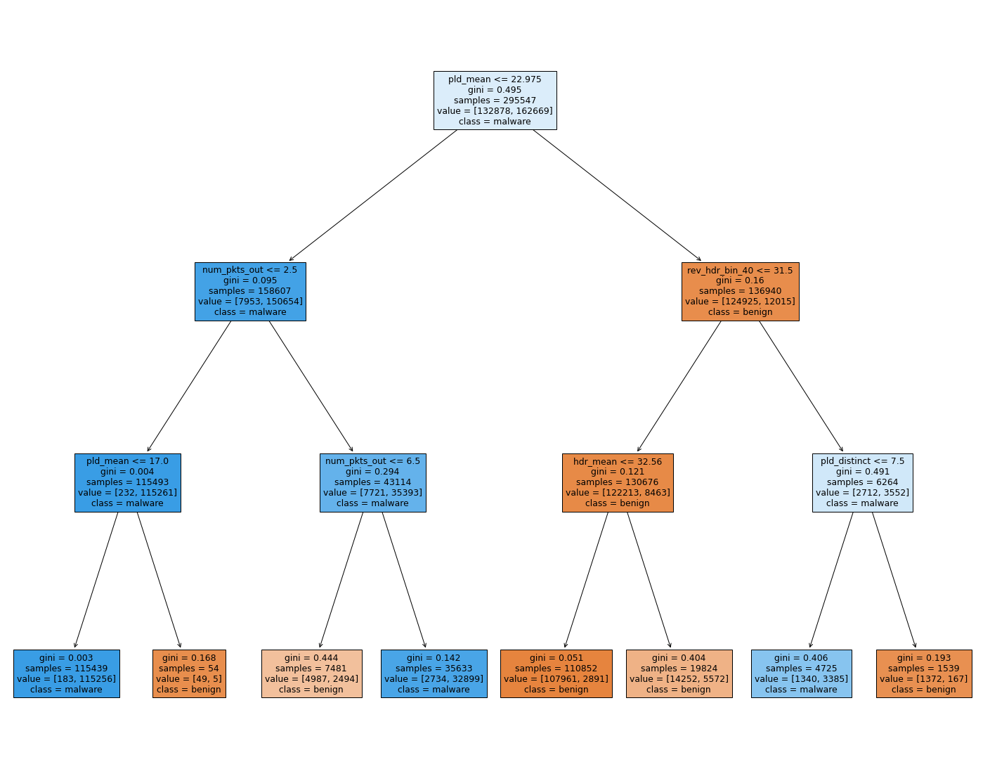
We are going to use a decision tree classifier since it is very visual.
We set the maximum depth of the tree to 3, to plot it effectively
from sklearn import tree
clf = tree.DecisionTreeClassifier(max_depth=3, random_state=42)
lf = clf.fit(X_train, y_train)
from matplotlib import pyplot as plt

DO_PLOTTING = True
if DO_PLOTTING:
    fig = plt.figure(figsize=(25,20))
    _ = tree.plot_tree(clf,
                       feature_names=train.columns[:FEATURE_TO_CONSIDER],
                       class_names=class_names,
                       filled=True)
    #fig.savefig("decistion_tree.png")
# let's predict the test test
test_pred_decision_tree = clf.predict(X_test)
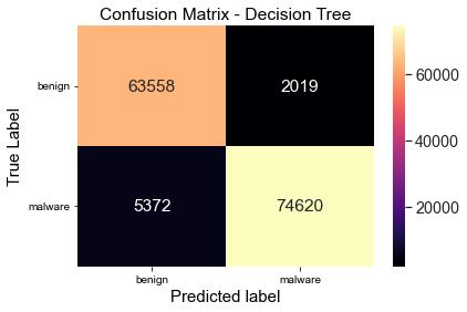
Evaluate the results
First with a confusion matrix to get a quick view.
Then using conventional metrics (accuracy, f1 etc).
#get the confusion matrix

from sklearn import metrics
import seaborn as sns
import matplotlib.pyplot as plt


confusion_matrix = metrics.confusion_matrix(y_test,
                                            test_pred_decision_tree)#turn this into a dataframe
matrix_df = pd.DataFrame(confusion_matrix)#plot the result
ax = plt.axes()
sns.set(font_scale=1.3)
plt.figure(figsize=(10,7))
sns.heatmap(matrix_df, annot=True, fmt="g", ax=ax, cmap="magma")#set axis titles
ax.set_title('Confusion Matrix - Decision Tree')
ax.set_xlabel("Predicted label", fontsize =15)
ax.set_xticklabels(['']+class_names)
ax.set_ylabel("True Label", fontsize=15)
ax.set_yticklabels(list(class_names), rotation = 0)
plt.show()
<Figure size 720x504 with 0 Axes>
# then with the

from sklearn import metrics

print(metrics.classification_report(y_test,
                                    test_pred_decision_tree))
              precision    recall  f1-score   support

           0       0.92      0.97      0.95     65577
           1       0.97      0.93      0.95     79992

    accuracy                           0.95    145569
   macro avg       0.95      0.95      0.95    145569
weighted avg       0.95      0.95      0.95    145569